Network histogram estimation for single-layer networks

Estimating a network histogram for a single-layer network and returning the indices of partitions.

Usage

nethist(A, h = NA, method = "PLL", control = nethist_control(), ...)

Arguments

A: An adjacency matrix or graph object. Accepted formats: a matrix, sparse dgCMatrix, igraph object, or network object. Must be an undirected simple graph.
h: A bandwidth parameter. If NA, the bandwidth is selected by Olhede and Wolfe (2014). If specified, the user-supplied value is used.
method: Type of loss function. One of "PLL" (default, profile log-likelihood) or "LSE" (least squares). See Details.
control: A control object from nethist_control. Governs max_itr, greedy_swap_rule, greedy_stop_threshold, and verbose.
...: Pass max_itr, greedy_swap_rule, greedy_stop_threshold, or verbose via control = nethist_control(...) instead.

Value

An object of class "nethist" with the following fields:

cluster an integer vector of length \(n\) with block assignments.
thetahat a \(k \times k\) probability matrix ordered by group labels.
rho_hat estimated sparsity parameter.
normalized_LL normalized log-likelihood.
MSE mean squared error.
method loss function used ("PLL" or "LSE").
h bandwidth used for estimation.

Details

method = "PLL" is for Olhede and Wolfe (2014). method = "LSE" is for Gao et al. (2015).

Note that cluster labels are not ordered: vertices in cluster 1 are not necessarily more similar to cluster 2 than to cluster 10. Users may specify a custom display order in plot.nethist.

References

Olhede, S. C. & Wolfe, P. J. (2014). Network Histograms and Universality of Blockmodel Approximation. PNAS, 111(41), 14722-14727. doi:10.1073/pnas.1400374111

Gao, C., Lu, Y., & Zhou, H. H. (2015). Rate-Optimal Graphon Estimation. The Annals of Statistics, 43(6), 2624-2652. doi:10.1214/15-AOS1354

Examples

# \donttest{
set.seed(42)
data(polblog)
fit <- nethist(polblog)
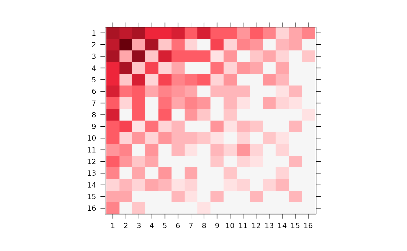
fit
#> 
#> thetahat:
#>               [,1]         [,2]         [,3]         [,4]         [,5]
#>  [1,] 0.2640791476 0.2203039970 0.2550197035 0.1131544380 0.1212234941
#>  [2,] 0.2203039970 0.6126331811 0.0108838431 0.2537061362 0.0026271345
#>  [3,] 0.2550197035 0.0108838431 0.3306697108 0.0022518296 0.1399887409
#>  [4,] 0.1131544380 0.2537061362 0.0022518296 0.0825722983 0.0007506099
#>  [5,] 0.1212234941 0.0026271345 0.1399887409 0.0007506099 0.0814307458
#>  [6,] 0.1392381310 0.0352786639 0.0568586977 0.0086320135 0.0272096078
#>  [7,] 0.0653030587 0.0011259148 0.0516044286 0.0000000000 0.0424094577
#>  [8,] 0.1366109964 0.0000000000 0.0658660161 0.0000000000 0.0561080878
#>  [9,] 0.0660536686 0.0964533684 0.0003753049 0.0373428411 0.0007506099
#> [10,] 0.0572340026 0.0005629574 0.0180146369 0.0009382623 0.0150121974
#> [11,] 0.0182022894 0.0225182961 0.0000000000 0.0151998499 0.0000000000
#> [12,] 0.0474760743 0.0191405517 0.0015012197 0.0091949709 0.0000000000
#> [13,] 0.0210170764 0.0000000000 0.0088196660 0.0000000000 0.0151998499
#> [14,] 0.0009382623 0.0037530494 0.0007506099 0.0071307938 0.0033777444
#> [15,] 0.0063801839 0.0061925314 0.0000000000 0.0000000000 0.0000000000
#> [16,] 0.0216629500 0.0000000000 0.0025485824 0.0000000000 0.0000000000
#>               [,6]         [,7]         [,8]         [,9]        [,10]
#>  [1,] 0.1392381310 0.0653030587 0.1366109964 0.0660536686 0.0572340026
#>  [2,] 0.0352786639 0.0011259148 0.0000000000 0.0964533684 0.0005629574
#>  [3,] 0.0568586977 0.0516044286 0.0658660161 0.0003753049 0.0180146369
#>  [4,] 0.0086320135 0.0000000000 0.0000000000 0.0373428411 0.0009382623
#>  [5,] 0.0272096078 0.0424094577 0.0561080878 0.0007506099 0.0150121974
#>  [6,] 0.0152207002 0.0061925314 0.0000000000 0.0031900919 0.0045036592
#>  [7,] 0.0061925314 0.0308219178 0.0125727153 0.0000000000 0.0048789642
#>  [8,] 0.0000000000 0.0125727153 0.0019025875 0.0000000000 0.0024394821
#>  [9,] 0.0031900919 0.0000000000 0.0000000000 0.0163622527 0.0001876525
#> [10,] 0.0045036592 0.0048789642 0.0024394821 0.0001876525 0.0000000000
#> [11,] 0.0050666166 0.0001876525 0.0000000000 0.0030024395 0.0009382623
#> [12,] 0.0000000000 0.0000000000 0.0000000000 0.0026271345 0.0000000000
#> [13,] 0.0000000000 0.0067554888 0.0000000000 0.0000000000 0.0024394821
#> [14,] 0.0001876525 0.0009382623 0.0000000000 0.0000000000 0.0001876525
#> [15,] 0.0030024395 0.0001876525 0.0000000000 0.0035653969 0.0000000000
#> [16,] 0.0000000000 0.0000000000 0.0001061909 0.0000000000 0.0000000000
#>              [,11]        [,12]        [,13]        [,14]        [,15]
#>  [1,] 0.0182022894 0.0474760743 0.0210170764 0.0009382623 0.0063801839
#>  [2,] 0.0225182961 0.0191405517 0.0000000000 0.0037530494 0.0061925314
#>  [3,] 0.0000000000 0.0015012197 0.0088196660 0.0007506099 0.0000000000
#>  [4,] 0.0151998499 0.0091949709 0.0000000000 0.0071307938 0.0000000000
#>  [5,] 0.0000000000 0.0000000000 0.0151998499 0.0033777444 0.0000000000
#>  [6,] 0.0050666166 0.0000000000 0.0000000000 0.0001876525 0.0030024395
#>  [7,] 0.0001876525 0.0000000000 0.0067554888 0.0009382623 0.0001876525
#>  [8,] 0.0000000000 0.0000000000 0.0000000000 0.0000000000 0.0000000000
#>  [9,] 0.0030024395 0.0026271345 0.0000000000 0.0000000000 0.0035653969
#> [10,] 0.0009382623 0.0000000000 0.0024394821 0.0001876525 0.0000000000
#> [11,] 0.0152207002 0.0007506099 0.0000000000 0.0007506099 0.0000000000
#> [12,] 0.0007506099 0.0003805175 0.0000000000 0.0000000000 0.0031900919
#> [13,] 0.0000000000 0.0000000000 0.0000000000 0.0009382623 0.0000000000
#> [14,] 0.0007506099 0.0000000000 0.0009382623 0.0041856925 0.0000000000
#> [15,] 0.0000000000 0.0031900919 0.0000000000 0.0000000000 0.0030441400
#> [16,] 0.0000000000 0.0000000000 0.0000000000 0.0000000000 0.0000000000
#>              [,16]
#>  [1,] 0.0216629500
#>  [2,] 0.0000000000
#>  [3,] 0.0025485824
#>  [4,] 0.0000000000
#>  [5,] 0.0000000000
#>  [6,] 0.0000000000
#>  [7,] 0.0000000000
#>  [8,] 0.0001061909
#>  [9,] 0.0000000000
#> [10,] 0.0000000000
#> [11,] 0.0000000000
#> [12,] 0.0000000000
#> [13,] 0.0000000000
#> [14,] 0.0000000000
#> [15,] 0.0000000000
#> [16,] 0.0000000000
#> 
#> Method: Profile Likelihood
#> 
#> normalized likelihood:
#> -3.05275785402995
#> 
#> Available components:
#> 
#> [1] "cluster"       "thetahat"      "rho_hat"       "normalized_LL"
#> [5] "MSE"           "method"        "h"            
plot(fit)


fit_h <- nethist(polblog, h = 72)
# }